前面介绍了K近邻算法,本节课用K近邻算法来做一个机器学习案例。
现在,这里有一些乳腺癌肿瘤的特征数据,我们需要根据这些特征数据来预测乳腺癌肿瘤是良性还是恶性,也就是说这是一个分类问题,而且是二分类问题。
乳腺癌肿瘤数据集介绍
首先,需要知道的是,每个肿瘤有以下10个特征:
- 半径(从中心到周边点的距离的平均值)
- 纹理(灰度值的标准偏差)
- 周边
- 面积
- 平滑度(半径长度的局部变化)
- 紧密度(周长^ 2 /面积-1.0)
- 凹度(轮廓的凹入部分的严重程度)
- 凹点(轮廓的凹入部分的数量)
- 对称性
- 分形维数(“海岸线近似”-1)
然后,计算出肿瘤的每个特征的的均值(mean)、标准差(standard error)和最差的(worst),也就是说每个特征对应三个数值型的值,所以每个肿瘤有30个特征,均为数值型。
这里的均值、标准差都好理解,最差的如何理解呢?
最差的表示肿瘤最糟的或最坏的,即某个特征,它的值越大/越小,肿瘤就越糟糕。
每个肿瘤有一个类别标签,恶性(Malignant)或者良性(Benign)。
肿瘤样本个数为569个。
代码实现
在理解了数据的基础上,接下来通过代码来实现。
数据集导入
首先,将数据集导入。
from sklearn.datasets import load_breast_cancer
cancer=load_breast_cancer()
通过DESCR查看数据描述信息。
print(cancer.DESCR) #等价于print(cancer['DESCR'])
运行结果:
.. _breast_cancer_dataset:

Breast cancer wisconsin (diagnostic) dataset
--------------------------------------------

**Data Set Characteristics:**

    :Number of Instances: 569

    :Number of Attributes: 30 numeric, predictive attributes and the class

    :Attribute Information:
        - radius (mean of distances from center to points on the perimeter)
        - texture (standard deviation of gray-scale values)
        - perimeter
        - area
        - smoothness (local variation in radius lengths)
        - compactness (perimeter^2 / area - 1.0)
        - concavity (severity of concave portions of the contour)
        - concave points (number of concave portions of the contour)
        - symmetry
        - fractal dimension ("coastline approximation" - 1)

        The mean, standard error, and "worst" or largest (mean of the three
        worst/largest values) of these features were computed for each image,
        resulting in 30 features.  For instance, field 0 is Mean Radius, field
        10 is Radius SE, field 20 is Worst Radius.

        - class:
                - WDBC-Malignant
                - WDBC-Benign

    :Summary Statistics:

    ===================================== ====== ======
                                           Min    Max
    ===================================== ====== ======
    radius (mean):                        6.981  28.11
    texture (mean):                       9.71   39.28
    perimeter (mean):                     43.79  188.5
    area (mean):                          143.5  2501.0
    smoothness (mean):                    0.053  0.163
    compactness (mean):                   0.019  0.345
    concavity (mean):                     0.0    0.427
    concave points (mean):                0.0    0.201
    symmetry (mean):                      0.106  0.304
    fractal dimension (mean):             0.05   0.097
    radius (standard error):              0.112  2.873
    texture (standard error):             0.36   4.885
    perimeter (standard error):           0.757  21.98
    area (standard error):                6.802  542.2
    smoothness (standard error):          0.002  0.031
    compactness (standard error):         0.002  0.135
    concavity (standard error):           0.0    0.396
    concave points (standard error):      0.0    0.053
    symmetry (standard error):            0.008  0.079
    fractal dimension (standard error):   0.001  0.03
    radius (worst):                       7.93   36.04
    texture (worst):                      12.02  49.54
    perimeter (worst):                    50.41  251.2
    area (worst):                         185.2  4254.0
    smoothness (worst):                   0.071  0.223
    compactness (worst):                  0.027  1.058
    concavity (worst):                    0.0    1.252
    concave points (worst):               0.0    0.291
    symmetry (worst):                     0.156  0.664
    fractal dimension (worst):            0.055  0.208
    ===================================== ====== ======

    :Missing Attribute Values: None

    :Class Distribution: 212 - Malignant, 357 - Benign

此处省略一万字......
以上描述性信息,前面已经介绍过了,这里就不多说了。
查看数据的前5条记录。
cancer.data[:5]
运行结果:
array([[1.799e+01, 1.038e+01, 1.228e+02, 1.001e+03, 1.184e-01, 2.776e-01,
        3.001e-01, 1.471e-01, 2.419e-01, 7.871e-02, 1.095e+00, 9.053e-01,
        8.589e+00, 1.534e+02, 6.399e-03, 4.904e-02, 5.373e-02, 1.587e-02,
        3.003e-02, 6.193e-03, 2.538e+01, 1.733e+01, 1.846e+02, 2.019e+03,
        1.622e-01, 6.656e-01, 7.119e-01, 2.654e-01, 4.601e-01, 1.189e-01],
       [2.057e+01, 1.777e+01, 1.329e+02, 1.326e+03, 8.474e-02, 7.864e-02,
        8.690e-02, 7.017e-02, 1.812e-01, 5.667e-02, 5.435e-01, 7.339e-01,
        3.398e+00, 7.408e+01, 5.225e-03, 1.308e-02, 1.860e-02, 1.340e-02,
        1.389e-02, 3.532e-03, 2.499e+01, 2.341e+01, 1.588e+02, 1.956e+03,
        1.238e-01, 1.866e-01, 2.416e-01, 1.860e-01, 2.750e-01, 8.902e-02],
       [1.969e+01, 2.125e+01, 1.300e+02, 1.203e+03, 1.096e-01, 1.599e-01,
        1.974e-01, 1.279e-01, 2.069e-01, 5.999e-02, 7.456e-01, 7.869e-01,
        4.585e+00, 9.403e+01, 6.150e-03, 4.006e-02, 3.832e-02, 2.058e-02,
        2.250e-02, 4.571e-03, 2.357e+01, 2.553e+01, 1.525e+02, 1.709e+03,
        1.444e-01, 4.245e-01, 4.504e-01, 2.430e-01, 3.613e-01, 8.758e-02],
       [1.142e+01, 2.038e+01, 7.758e+01, 3.861e+02, 1.425e-01, 2.839e-01,
        2.414e-01, 1.052e-01, 2.597e-01, 9.744e-02, 4.956e-01, 1.156e+00,
        3.445e+00, 2.723e+01, 9.110e-03, 7.458e-02, 5.661e-02, 1.867e-02,
        5.963e-02, 9.208e-03, 1.491e+01, 2.650e+01, 9.887e+01, 5.677e+02,
        2.098e-01, 8.663e-01, 6.869e-01, 2.575e-01, 6.638e-01, 1.730e-01],
       [2.029e+01, 1.434e+01, 1.351e+02, 1.297e+03, 1.003e-01, 1.328e-01,
        1.980e-01, 1.043e-01, 1.809e-01, 5.883e-02, 7.572e-01, 7.813e-01,
        5.438e+00, 9.444e+01, 1.149e-02, 2.461e-02, 5.688e-02, 1.885e-02,
        1.756e-02, 5.115e-03, 2.254e+01, 1.667e+01, 1.522e+02, 1.575e+03,
        1.374e-01, 2.050e-01, 4.000e-01, 1.625e-01, 2.364e-01, 7.678e-02]])
说明:因为特征较多,所以数据看起来很多!
通过shape查看特征数据的形状。
cancer.data.shape
运行结果:
(569, 30)
569个样本,30个特征。
通过feature_names查看特征名称。
cancer.feature_names
运行结果:
array(['mean radius', 'mean texture', 'mean perimeter', 'mean area',
       'mean smoothness', 'mean compactness', 'mean concavity',
       'mean concave points', 'mean symmetry', 'mean fractal dimension',
       'radius error', 'texture error', 'perimeter error', 'area error',
       'smoothness error', 'compactness error', 'concavity error',
       'concave points error', 'symmetry error',
       'fractal dimension error', 'worst radius', 'worst texture',
       'worst perimeter', 'worst area', 'worst smoothness',
       'worst compactness', 'worst concavity', 'worst concave points',
       'worst symmetry', 'worst fractal dimension'], dtype='<U23')
这里的名称也不多解释了,中文翻译见PPT。
通过target查看样本的类别标签。
cancer.target[:20]
运行结果:
array([0, 0, 0, 0, 0, 0, 0, 0, 0, 0, 0, 0, 0, 0, 0, 0, 0, 0, 0, 1])
说明:0代表良性,1代表恶性。
通过target_names查看类别标签的名称。
cancer.target_names
运行结果:
array(['malignant', 'benign'], dtype='<U9')
将数据集拆分成训练集和测试集
调用train_test_split函数将数据集拆分成训练集和测试集。
from sklearn.model_selection import train_test_split
X_train,X_test,y_train,y_test=train_test_split(cancer.data,cancer.target,random_state=0)
这里没有设置比例,默认test_size=0.25,即数据集的75%是训练集,剩余25%是测试集。
用训练集去训练K近邻算法
from sklearn.neighbors import KNeighborsClassifier
clf=KNeighborsClassifier(n_neighbors=3)
clf.fit(X_train,y_train)
运行结果:
KNeighborsClassifier(n_neighbors=3)
这里调用K近邻算法,设置K=3。
根据测试集的精度评估模型
clf.score(X_test,y_test)
运行结果:
0.9230769230769231
此时,测试集的进度约为0.92。
如何选择K值?
我们知道,对于K近邻算法来说,参数只有一个K,所以K值的选择对于模型的精度会有影响,那么,如何选择合适的K值呢?
我们的方法是通过循环去测试多个K值,然后选择泛化精度最高的那个K值,代码实现如下。
#以n_neighbors为自变量,对比训练集精度和测试集精度
from sklearn.datasets import load_breast_cancer
import matplotlib.pyplot as plt

cancer=load_breast_cancer()
X_train,X_test,y_train,y_test=train_test_split(cancer.data,cancer.target,stratify=cancer.target,random_state=66)
#参数stratify: 依据标签y,按原数据y中各类比例,分配给train和test,使得train和test中各类数据的比例与原数据集一样。
training_accuracy=[]
test_accuracy=[]
#n_neighbors取值从1到10
neighbors_settings=range(1,11)

for n_neighbors in neighbors_settings:
    clf=KNeighborsClassifier(n_neighbors=n_neighbors)
    clf.fit(X_train,y_train)
    #记录训练集精度
    training_accuracy.append(clf.score(X_train,y_train))
    #记录泛化精度
    test_accuracy.append(clf.score(X_test,y_test))

plt.plot(neighbors_settings,training_accuracy,label="trainingaccuracy")
plt.plot(neighbors_settings,test_accuracy,label="testaccuracy")
plt.ylabel("Accuracy")
plt.xlabel("n_neighbors")
plt.legend()
plt.show()
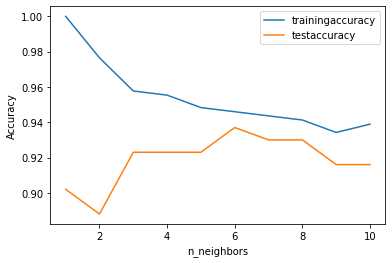
在以上代码中,对不同K值的训练集精度和泛化精度进行了可视化展示,通过这个曲线图可以看出,当K=6时,泛化精度最高,此时,测试集的进度也在一个比较理想的状态,所以选择K=6即可。
好了,这就是用K近邻算法去预测乳腺癌。